Band-by-Band

Comparing how ‘Band-by-Band’ approaches relate to periodic & aperiodic components.

This example is based on a recent project investigating band-by-band analyses as often done in the context of development. The paper for that project is available here.

# Import numpy and matplotlib
import numpy as np
import matplotlib.pyplot as plt

# Import the FOOOF object
from fooof import FOOOF

# Import simulation, utility, and plotting tools
from fooof.bands import Bands
from fooof.utils import trim_spectrum
from fooof.analysis import get_band_peak_fm
from fooof.sim.gen import gen_power_spectrum
from fooof.sim.utils import set_random_seed
from fooof.plts.spectra import plot_spectra_shading

Overview

A common analysis approach for investigating neural data is to measure and analyze changes across multiple frequency bands.

This is typically done using predefined bands, such as:

• delta (1-4 Hz)

• theta (4-8 Hz)

• alpha (8-13 Hz)

• beta (13-30 Hz)

• gamma (30-50 Hz)

When analyzed in this way, and comparing within or between subjects, investigations often report a pattern of changes or differences across bands, for example:

• decreased power in lower frequency bands (delta, theta)

• increased power in higher frequency bands (beta, gamma)

Under this framework, each defined band reflects a different entity in the data, and the interpretation is typically that there are multiple things changing, with correlated changes in power across multiple distinct bands.

An alternative hypothesis for what is changing is that this pattern of results could be driven by changes or differences in the aperiodic component of the data. Changes in aperiodic activity, when analyzed in a band-by-band manner, can look like correlated changes across multiple bands.

In this example, we will use simulated data to examine both the different ways of analyzing such data (band-by-band compared to parameterizing neural power spectra), and examine what it looks like if data differs in these hypothesized ways. To do so, we will simulate and analyze data with correlated changes in multiple distinct frequency bands, as well as data in which there is a shift in the aperiodic component.

Settings

First, we can define some settings for this notebook and analysis.

# Define our frequency bands of interest
bands = Bands({'delta' : [1, 4],
               'theta' : [4, 8],
               'alpha' : [8, 13],
               'beta' : [13, 30],
               'gamma' : [30, 50]})

# Define plot settings
t_settings = {'fontsize' : 24, 'fontweight' : 'bold'}
shade_cols = ['#e8dc35', '#46b870', '#1882d9', '#a218d9', '#e60026']
labels = ['Group-1', 'Group-2']

# General simulation settings
f_range = [1, 50]
nlv = 0

# Define some template strings for reporting
exp_template = "The difference of aperiodic exponent is: \t {:1.2f}"
pw_template = ("The difference of {:5} power is  {: 1.2f}\t"
               "with peaks or  {: 1.2f}\t with bands.")

Helper Functions

Throughout this notebook we will be computing and analyzing differences between power spectra. Here, we will define some helper functions to do so.

def compare_exp(fm1, fm2):
    """Compare exponent values."""

    exp1 = fm1.get_params('aperiodic_params', 'exponent')
    exp2 = fm2.get_params('aperiodic_params', 'exponent')

    return exp1 - exp2

def compare_peak_pw(fm1, fm2, band_def):
    """Compare the power of detected peaks."""

    pw1 = get_band_peak_fm(fm1, band_def)[1]
    pw2 = get_band_peak_fm(fm2, band_def)[1]

    return pw1 - pw2

def compare_band_pw(fm1, fm2, band_def):
    """Compare the power of frequency band ranges."""

    pw1 = np.mean(trim_spectrum(fm1.freqs, fm1.power_spectrum, band_def)[1])
    pw2 = np.mean(trim_spectrum(fm1.freqs, fm2.power_spectrum, band_def)[1])

    return pw1 - pw2

Band-by-Band

In the ‘band-by-band’ idea of the data, analyses and interpretations focus on analyzing activity across a range of frequency bands, and looking for patterns of changes within and between these bands.

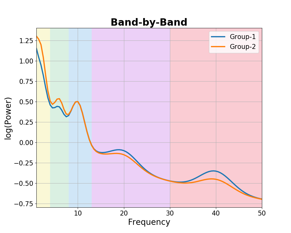
To visualize this, we can simulate hypothesized power spectra for different groups, in which we will set the same aperiodic activity, and vary overlying periodic peaks.

In this example, for clarity, the center frequencies for all peaks are simulated as being the same between groups, though in real data these could also vary.

# Set consistent aperiodic parameters
ap_params = [1, 1]

# Set periodic parameters, defined to vary between groups
#   All parameters are set to match, except for systematic power differences
pe_g1 = [[2, 0.25, 1], [6, 0.2, 1], [10, 0.5, 1.5], [20, 0.2, 3], [40, 0.25, 3.5]]
pe_g2 = [[2, 0.5, 1], [6, 0.3, 1], [10, 0.5, 1.5], [20, 0.15, 3], [40, 0.15, 3.5]]

# Set random seed, for consistency generating simulated data
set_random_seed(21)

# Simulate example power spectra for each group
freqs, g1_spectrum_bands = gen_power_spectrum(f_range, ap_params, pe_g1, nlv)
freqs, g2_spectrum_bands = gen_power_spectrum(f_range, ap_params, pe_g2, nlv)

# Plot the power spectra differences, representing the 'band-by-band' idea
plot_spectra_shading(freqs, [g1_spectrum_bands, g2_spectrum_bands],
                     log_powers=True, linewidth=3,
                     shades=bands.definitions, shade_colors=shade_cols,
                     labels=labels)
plt.xlim(f_range);
plt.title('Band-by-Band', t_settings);

Out:

Text(0.5, 1.0, 'Band-by-Band')

Flatten the Spectra

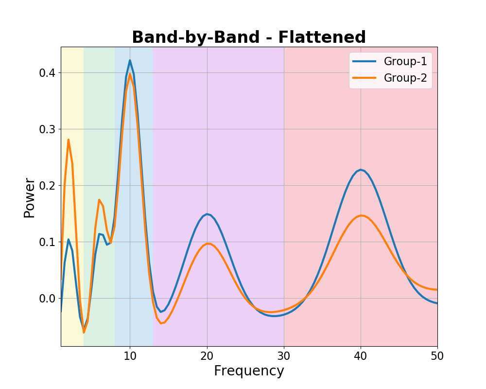
Under the band-by-band idea, controlling for aperiodic activity and flattening the spectra should show specific differences in each band.

It should also find no systematic difference in the aperiodic activity between groups.

To check this, we can fit power spectrum models, and examine which parameters are changing in the data.

# Initialize FOOOF objects
fm_bands_g1 = FOOOF(verbose=False)
fm_bands_g2 = FOOOF(verbose=False)

# Fit power spectrum models
fm_bands_g1.fit(freqs, g1_spectrum_bands)
fm_bands_g2.fit(freqs, g2_spectrum_bands)

# Plot the power spectra differences
plot_spectra_shading(freqs, [fm_bands_g1._spectrum_flat, fm_bands_g2._spectrum_flat],
                     log_powers=False, linewidth=3,
                     shades=bands.definitions, shade_colors=shade_cols,
                     labels=labels)
plt.xlim(f_range);
plt.title('Band-by-Band - Flattened', t_settings);

Out:

Text(0.5, 1.0, 'Band-by-Band - Flattened')

Compare Spectral Parameters

Next, let’s compare the measured parameters of the data.

# Check the difference of aperiodic activity between age groups
print(exp_template.format(compare_exp(fm_bands_g1, fm_bands_g2)))

Out:

The difference of aperiodic exponent is:         -0.07

# Check the difference in periodic activity, across bands, between groups
for label, definition in bands:
    print(pw_template.format(label,
                             compare_peak_pw(fm_bands_g1, fm_bands_g2, definition),
                             compare_band_pw(fm_bands_g1, fm_bands_g2, definition)))

Out:

The difference of delta power is  -0.18 with peaks or  -0.16     with bands.
The difference of theta power is  -0.05 with peaks or  -0.06     with bands.
The difference of alpha power is   0.02 with peaks or  -0.00     with bands.
The difference of beta  power is   0.05 with peaks or   0.02     with bands.
The difference of gamma power is   0.08 with peaks or   0.04     with bands.

In the measurements above, we can see there is a negligible difference in the aperiodic properties of the data, but that there are differences within individual bands, with the same pattern of results highlighted by comparing either the parameterized peaks or the average band power.

This is as expected, given that we simulated the data to reflect this idea. In the simulation we can see that both a band-by-band analysis, and parameterizing neural power spectra give the same, and correct result for this case.

Periodic & Aperiodic

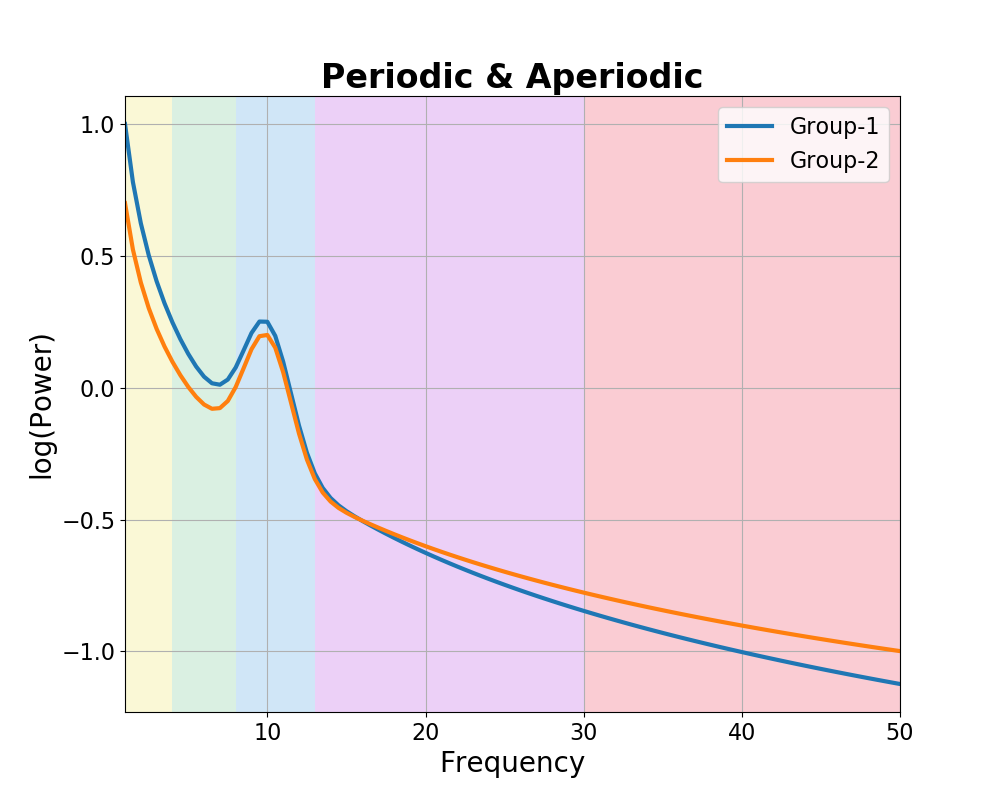
An alternative hypothesis is that aperiodic activity may vary between groups.

In the next simulation, we will simulate each group as having same periodic activity, in this case, just an alpha peak, with a difference in the aperiodic activity.

# Simulate spectra for each group, with aperiodic differences
freqs, g1_spectrum_pa = gen_power_spectrum(f_range, [1.0, 1.25], [10, 0.5, 1.5], nlv)
freqs, g2_spectrum_pa = gen_power_spectrum(f_range, [0.7, 1.00], [10, 0.5, 1.5], nlv)

# Plot the power spectra differences
plot_spectra_shading(freqs, [g1_spectrum_pa, g2_spectrum_pa],
                     log_freqs=False, log_powers=True, linewidth=3,
                     shades=bands.definitions, shade_colors=shade_cols,
                     labels=labels)
plt.xlim(f_range);
plt.title('Periodic & Aperiodic', t_settings);

Out:

Text(0.5, 1.0, 'Periodic & Aperiodic')

Flatten the Spectra

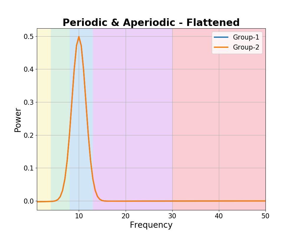
In the scenario in which there are differences in aperiodic activity, flattening the spectra should show no differences in periodic peaks.

We can again parameterize the spectra to investigate this.

# Initialize FOOOF objects
fm_pa_g1 = FOOOF(verbose=False)
fm_pa_g2 = FOOOF(verbose=False)

# Fit power spectrum models
fm_pa_g1.fit(freqs, g1_spectrum_pa)
fm_pa_g2.fit(freqs, g2_spectrum_pa)

# Plot the power spectra differences
plot_spectra_shading(freqs, [fm_pa_g1._spectrum_flat, fm_pa_g2._spectrum_flat],
                     log_powers=False, linewidth=3,
                     shades=bands.definitions, shade_colors=shade_cols,
                     labels=labels)
plt.xlim(f_range);
plt.title('Periodic & Aperiodic - Flattened', t_settings);

Out:

Text(0.5, 1.0, 'Periodic & Aperiodic - Flattened')

Compare Spectral Parameters

Let’s again compare the measured parameters of the data.

# Check the difference of aperiodic activity between age groups
print(exp_template.format(compare_exp(fm_pa_g1, fm_pa_g2)))

Out:

The difference of aperiodic exponent is:         0.25

# Check the difference in periodic activity, across bands, between groups
for label, definition in bands:
    print(pw_template.format(label,
                             compare_peak_pw(fm_pa_g1, fm_pa_g2, definition),
                             compare_band_pw(fm_pa_g1, fm_pa_g2, definition)))

Out:

The difference of delta power is   nan  with peaks or   0.21     with bands.
The difference of theta power is   nan  with peaks or   0.11     with bands.
The difference of alpha power is   0.00 with peaks or   0.05     with bands.
The difference of beta  power is   nan  with peaks or  -0.03     with bands.
The difference of gamma power is   nan  with peaks or  -0.10     with bands.

In the measurements above, we can now see that we are measuring a difference in the aperiodic properties of the data.

We also see a different results when looking at bands / peaks, depending on how we analyze them. The band-by-band analysis reports a pattern of differences across the frequency bands. However, the parameterized analysis reports no differences in identified peaks.

Note that when comparing peaks, ‘nan’ reflects that there were no identified peaks to compare, where are a zero value reflects that peaks were detected, but they did not differ.

In this case, we know that the parameterization approach results in the correct interpretation of the changes in the data.

Conclusion

Here we have investigated changes across power spectra, comparing a ‘band-by-band’ approach to the parameterizing neural power spectra notion of ‘periodic & aperiodic’ components.

What we can see is that parameterizing neural power spectra is able to determine if changes are driven by differences in oscillatory peaks, and/or by changes in the aperiodic component of the data.

However, we also saw that simply doing a band-by-band power analysis can conflate differences from aperiodic and periodic changes. Specifically, when we change the aperiodic activity in a power spectrum, the band-by-band analysis suggests that multiple distinct frequency bands are changing, whereas the more parsimonious (and in the simulated case, the true) conclusion should be that changes are driven by changes in the aperiodic activity that affects all frequencies. This also means that if a band-by-band analysis finds differences across bands, this is not enough to know if there are band-specific changes, or aperiodic changes, as this analysis approach does not differentiate the two.

We conclude here that band-by-band analysis, without measuring or controlling for aperiodic activity, are ill posed to adjudicate which aspects of the data are changing. Parameterizing neural power spectra allows for disentangling changes in periodic and aperiodic components of the data.

In this example, with simulated data, we cannot conclude which changes are more likely to be occurring in real data. However, in the real data analysis that this example is based on, it was found that a great deal of the changes across development are driven by aperiodic changes, and not by band-by-band differences. This finding came from using the parameterization approach, but was not evidence in prior work using only a band-by-band approach. You can find more on that project here.